Dijkstra's shortest path, visually

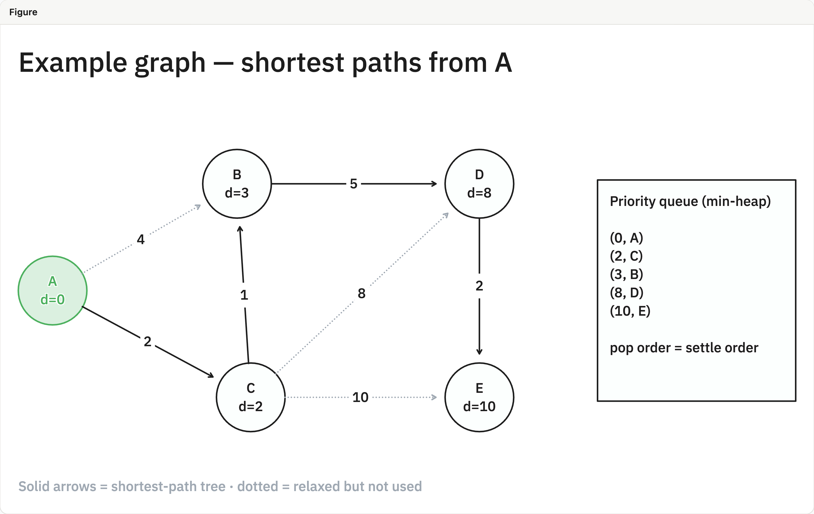
Dijkstra's algorithm finds the cheapest path from one source to every other node in a graph with non-negative edge weights. The canvas shows the example graph; the note walks through it step by step.

The idea in one sentence

Always settle the closest unsettled node next. Its distance can never improve later, because every other route is already at least as long.

Relaxation

For an edge $u \to v$ with weight $w(u,v)$, relaxing it means:

Code

import heapq

def dijkstra(graph, source):
    dist = {node: float("inf") for node in graph}
    dist[source] = 0
    heap = [(0, source)]
    while heap:
        d, u = heapq.heappop(heap)
        if d > dist[u]:
            continue  # stale entry
        for v, w in graph[u]:
            if d + w < dist[v]:
                dist[v] = d + w
                heapq.heappush(heap, (dist[v], v))
    return dist

Worked trace from A

1. Settle A (0). Relax: B = 4, C = 2.
2. Settle C (2). Relax: B = min(4, 2+1) = 3, D = 2+8 = 10, E = 2+10 = 12.
3. Settle B (3). Relax: D = min(10, 3+5) = 8.
4. Settle D (8). Relax: E = min(12, 8+2) = 10.
5. Settle E (10). Done.

Final distances: A 0 · B 3 · C 2 · D 8 · E 10.

flowchart LR
  A((A)) -- 4 --> B((B))
  A -- 2 --> C((C))
  C -- 1 --> B
  B -- 5 --> D((D))
  C -- 8 --> D
  C -- 10 --> E((E))
  D -- 2 --> E

Complexity

With a binary heap each edge can push once and each pop costs $\log V$:

Common mistakes

• Using it with negative weights. Use Bellman–Ford instead.
• Forgetting the stale entry check, which makes it slow on dense graphs.
• Marking a node visited when it is pushed instead of when it is popped.